Home › Lab 2
Lab 2: IMU
Overview
In this lab we tested the IMU sensor's range and quality, anaylizing both the accelerometer and gyro. We then took in data and tried various methods of process and transmitting it.
Lab Tasks
Set up the IMU
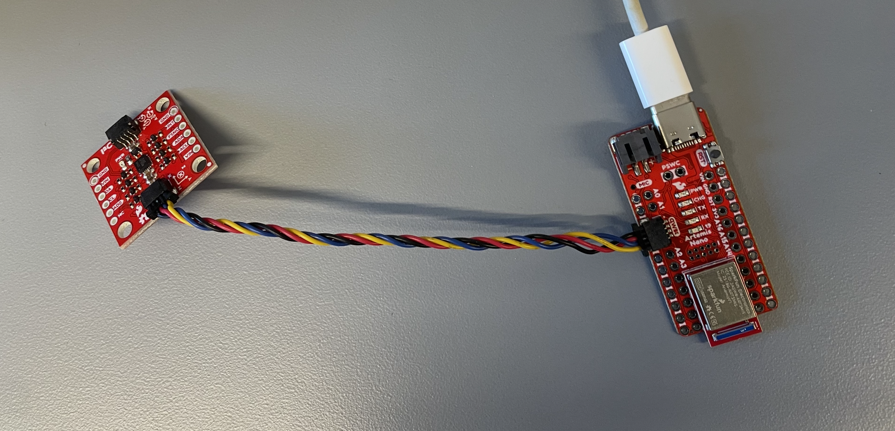
Figure: Artemis to IMU wiring using Qwiic connectors.
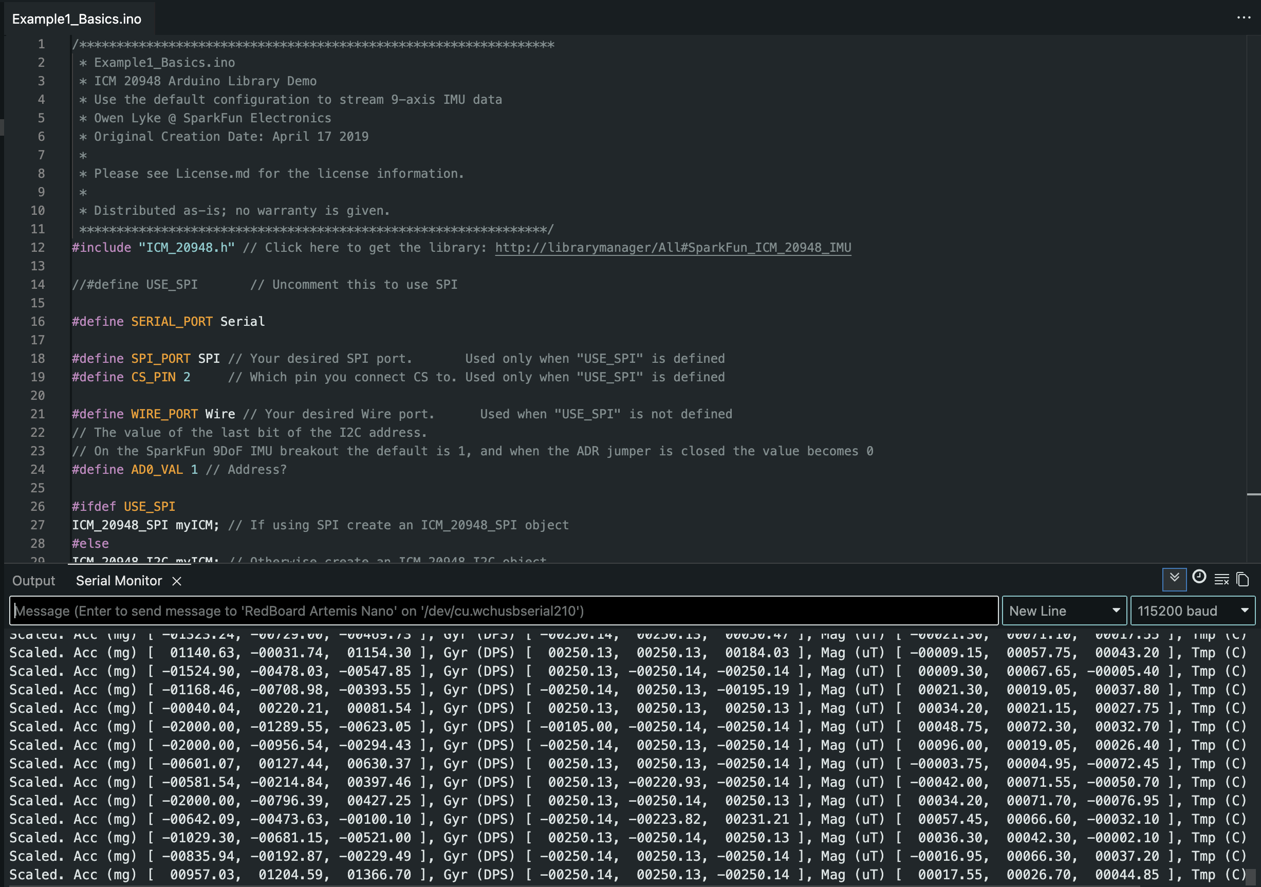
Figure: SparkFun ICM-20948 example running and producing sensor output.
AD0_VAL definition
The AD0_VAL definition is offered at two different locations with contrasting information. The sparkfun website says that it's by default 1, when the jumper is open, and the I2C address of the IMU is 0x69 (closed the IMU’s address is 0x68). In theory, the constant being one in the library's address (where the IMU is) should be that default value of 1 with the jumper open. However, the online data sheet contradicts this. Regardless though, in our sketchw w have #define AD0_VAL 1 anyway.
Acceleration and gyroscope data discussion
Here I shook the board and sensor in a quick jolt. You'll note that values 1-6 in the following screenshots are accX (mg), accY (mg), accZ (mg), gyrX (DPS), gyrY (DPS), and gyrZ (DPS) in order. The first shows the accelerometer detection, and then gyro after. It seems the change in the sensor values are already well dialed into the motion. Following that is an image of the code I used to blink the led 3 times on start up to indicate success.
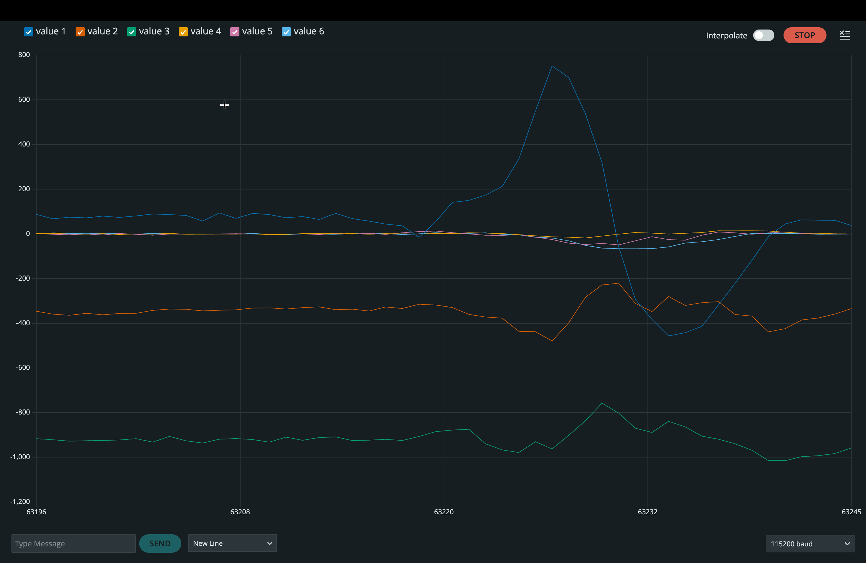
Figure: Example accelerometer data while rotating, flipping, and accelerating the board.
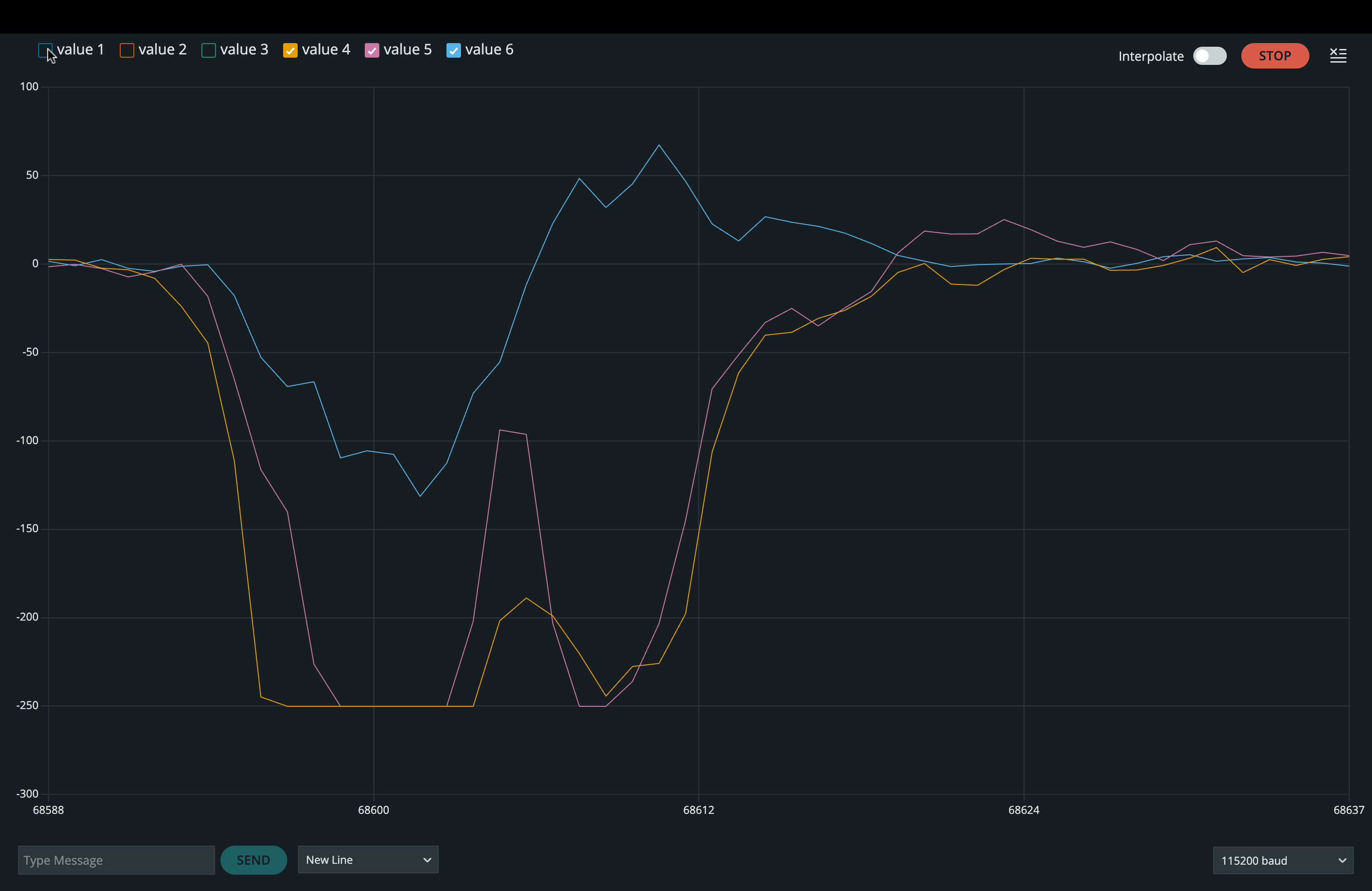
Figure: Example gyroscope data while rotating, flipping, and accelerating the board.
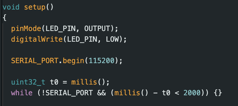
Figure: Startup running indicator implementation (three slow blinks).
Equations Used
Conventions and units
Variables: \(a_x, a_y, a_z\) are accelerometer readings along the IMU axes. \( \omega_x, \omega_y, \omega_z \) are gyroscope angular rates.
Time step: \(dt\) in seconds.
Angle units: compute in radians, convert to degrees for display.
deg = rad * 180.0 / π
rad = deg * π / 180.0
Pitch and roll from accelerometer
Use accelerometer gravity direction to estimate tilt. These forms won't break while using \(\operatorname{atan2}\).
\[
\text{roll}_{acc} = \operatorname{atan2}(a_y, a_z)
\]
\[
\text{pitch}_{acc} = \operatorname{atan2}\!\left(-a_x,\sqrt{a_y^2 + a_z^2}\right)
\]
Implementation mapping: \(a_x = \texttt{accX}\), \(a_y = \texttt{accY}\), \(a_z = \texttt{accZ}\) (any consistent units, mg is fine).
Gyroscope angle integration (pitch, roll, yaw)
Gyroscope gives angular rate. Integrate over time to get angle. This drifts over time.
\[
\theta_g[k] = \theta_g[k-1] + \omega[k]\;dt
\]
First order low-pass filter (used on accelerometer angle or raw accel)
Smooth noisy signals before fusion or for plotting.
\[
y[k] = \alpha\,y[k-1] + (1-\alpha)\,x[k]
\]
\[
\tau = \frac{1}{2\pi f_c}
\qquad
\alpha = \frac{\tau}{\tau + dt}
\]
\(f_c\) is the cutoff frequency in Hz chosen from your FFT analysis.
Complementary filter (accelerometer plus gyroscope)
Combines gyro short-term stability with accel long-term reference.
\[
\theta[k] = \beta\left(\theta[k-1] + \omega[k]\;dt\right) + (1-\beta)\,\theta_{acc}[k]
\]
\(\beta\) is typically close to 1 (example: 0.95 to 0.99). Use the same for the other two.
FFT frequency axis (for your Python spectrum plot)
Used to label the spectrum and justify \(f_c\). If your sampling rate is \(f_s\) and you collect \(N\) samples:
\[
f_s \approx \frac{1}{\operatorname{median}(\Delta t)}
\qquad
f[i] = \frac{i\,f_s}{N}, \; i = 0,1,\dots,\left\lfloor\frac{N}{2}\right\rfloor
\]
Accelerometer
Video: Pitch and roll output demonstration near -90, 0, +90 degrees with requested visual of output.
Accelerometer accuracy
Acceleromater accuracy was quite good, as evidenced by the video and double checked by a two point calibration as suggested.
Notes
The following plots use the same recorded dataset for time domain, FFT, and low pass filtering.
Noise in the Frequency Spectrum
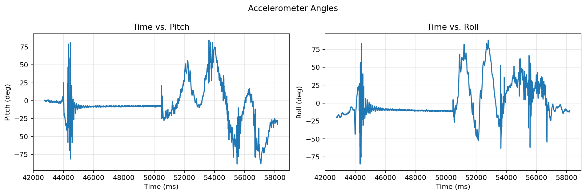
Accelerometer pitch and roll versus time.
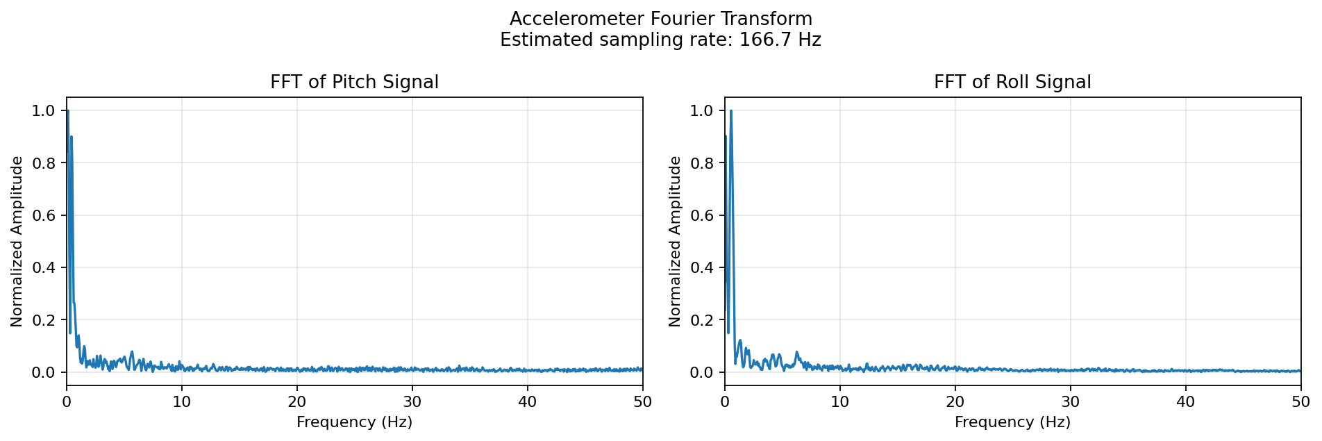
One sided FFT of accelerometer pitch and roll (normalized amplitude).
For data I rolled around the sensor in my hands at various angles and speeds to get data on natural vibrations from movement, and also let it be vibrated by the car. Then I performed the transform as instructed in class. The cutoff frequency I chose was 5 Hz because the FFT showed meaningful pitch and roll dynamics in the low-frequency band. All of the noise was higher, so this leaves the motion that is slow and intentional, rather than random vibrations. This choice was critical for processing sensor data and will be necessary to not lose information from the car’s movements in future labs. I then used a first order low pass filter to get the following.
Accelerometer Low Pass Filter
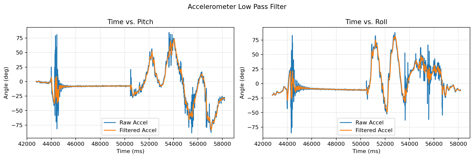
Raw accelerometer angles compared to low pass filtered angles.
Gyroscope
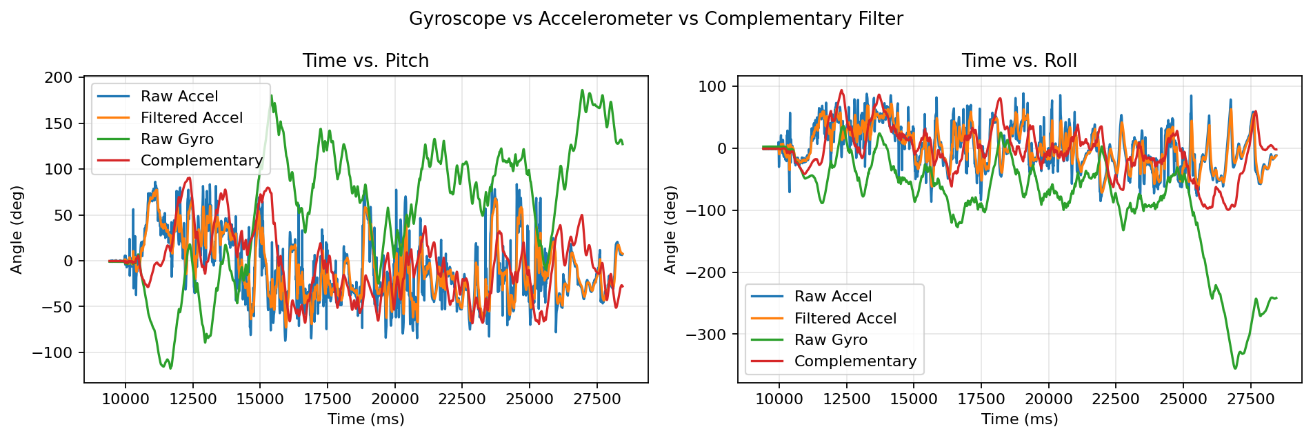
Pitch and roll: raw accel, filtered accel, integrated gyro, complementary filter.
In the graphs below you can see the results of the IMU being rolled around on the gyroscope data as well. You’ll note that it’s way more smooth than the accelerometer, but like mentioned in class, it’s much more susceptible to drifting over time. However, with good consistant sampling, you can keep a true dt value and have less error per step. When testing different sampling frequencies, we got a lot of error build up from it. The complementary filter I implemented was great, much more stable than the accelerometer and much less laggy than the low pass filter alone, as well as free of the gyro drift. I chose .98 for beta, and as you can see, it performed very well even under quick changes and a large variety angles and movements.
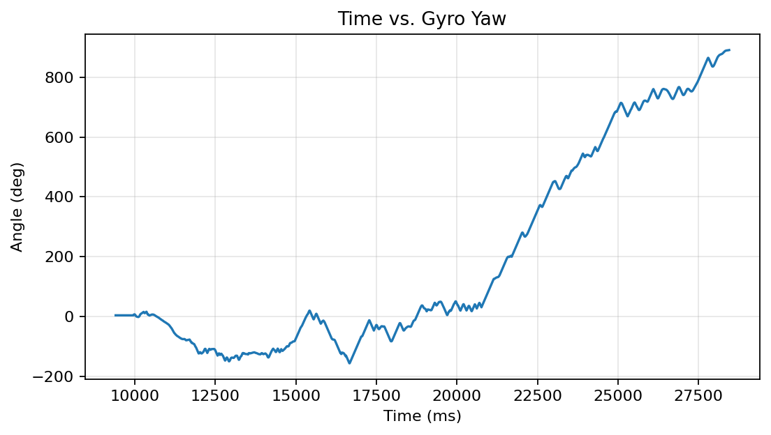
Yaw angle from gyroscope integration.
I finished up by creating the array and ensuring it would send via bluetooth using the following code.
    void record5s_to_arrays()
    {
      n = 0;
      uint32_t t0_ms = millis();
      uint32_t last_us = micros();

      while ((millis() - t0_ms) < RECORD_MS && n < MAX_SAMPLES)
      {
        if (!myICM.dataReady()) continue;

        myICM.getAGMT(); // updates myICM.agmt

        uint32_t now_us = micros();
        if ((uint32_t)(now_us - last_us) < SAMPLE_PERIOD_US) continue;
        last_us = now_us;

        t_ms[n] = millis() - t0_ms;

        ax_raw[n] = myICM.agmt.acc.axes.x;
        ay_raw[n] = myICM.agmt.acc.axes.y;
        az_raw[n] = myICM.agmt.acc.axes.z;

        gx_raw[n] = myICM.agmt.gyr.axes.x;
        gy_raw[n] = myICM.agmt.gyr.axes.y;
        gz_raw[n] = myICM.agmt.gyr.axes.z;

        n++;
      }
    }
The bluetooth fought me every step of the way.
    void bleSendChunked(const char* s)
    {
      while (*s)
      {
        uint8_t k = 0;
        char chunk[20];
        while (*s && k < 20) chunk[k++] = *s++;
        txChar.writeValue((const unsigned char*)chunk, k); // notify chunk
        delay(2); // small pacing helps it stop dropping info randomly
      }
    }

    void bleSendLine(const char* s)
    {
      bleSendChunked(s);
      bleSendChunked("\n");
    }

    void transmit_arrays_ble()
    {
      bleSendLine("H,t_ms,ax,ay,az,gx,gy,gz");
      char line[96];

      for (uint16_t i = 0; i < n; i++)
      {
        snprintf(line, sizeof(line),
                 "D,%lu,%d,%d,%d,%d,%d,%d",
                 (unsigned long)t_ms[i],
                 (int)ax_raw[i], (int)ay_raw[i], (int)az_raw[i],
                 (int)gx_raw[i], (int)gy_raw[i], (int)gz_raw[i]);
        bleSendLine(line);
      }

      bleSendLine("DUMP_END");
    }

  }
Record a Stunt
Video: Recorded stunt.
Here I played around and managed to get the car to go on it's side, which I think will introduce some difficulty later on in programing this car. I tested this all for about 10 minutes out on carpet, which the car actually was not very reliable on. I'm unsure if it was the type of carpet, but I expected it to skid around less. However, I tried various accelerations in straight lines, curves, and flips, and almost nothing went as intended. When accelerating, the wheels would often not catch proeprly on the carpet. Especially when turning, though, the car was entirely unpredictable. I tried driving a path, and then closing my eyes and trying to drive the same path (a loop through my friend's kitchen to the living room) and it was impossible to predict.
Credit in this lab: I used multiple past student's websites for guidance, especially on the coding and graphing sections to know what was appropriate/relevent to include and debug. I used chatgpt 5.2 to help me debug the generation of graphs, and help make the html for this website. Also, some stack overflow for figuring out errors.